iLQGames.jl

iLQGames.jl is a framework for rapidly designing and solving nonlinear general-sum differential games, built around iterative linear-quadratic game approximations.

A brief introduction to this framework and benchmarks against a C++ implementation can be found in this short workshop manuscript. Finally, this paper demonstrates the flexibility and performance of iLQGames.jl by combining it with a particle-filter scheme to reason about uncertainty in differential games in real-time.

Installation

Within the Julia REPL run:

using Pkg
Pkg.add(PackageSpec(url="https://github.com/lassepe/iLQGames.jl"))

Example

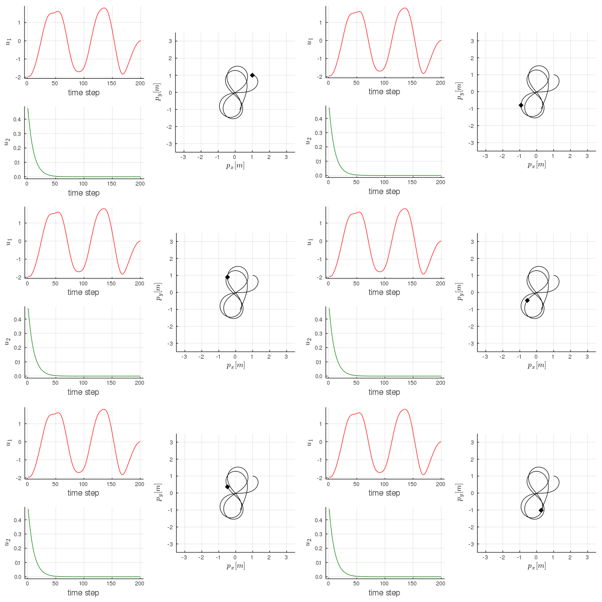
Here is an example of two players controlling a single 4D-unicycle. Player-1 controls the steering, Player-2 controls the acceleration.

1. Describe Dynamics

We define a Unicycle as a subtype of our ControlSystem type and implement the differential equation by overloading dx for our type.

using iLQGames
import iLQGames: dx

# parameters: number of states, number of inputs, sampling time, horizon
nx, nu, ΔT, game_horizon = 4, 2, 0.1, 200

# setup the dynamics
struct Unicycle <: ControlSystem{ΔT,nx,nu} end
# the differential equation of a uncycle with state: (px, py, phi, v)
dx(cs::Unicycle, x, u, t) = SVector(x[4]cos(x[3]), x[4]sin(x[3]), u[1], u[2])
dynamics = Unicycle()

2. Setup Costs

To setup the costs encoding each players objectives, we can derive a custom subtype from PlayerCost, or, as done here, simply hand the cost function as a lambda function to the FunctionPlayerCost.

# player-1 wants the unicycle to stay close to the origin,
# player-2 wants to keep close to 1 m/s
costs = (FunctionPlayerCost((g, x, u, t) -> (x[1]^2 + x[2]^2 + u[1]^2)),
         FunctionPlayerCost((g, x, u, t) -> ((x[4] - 1)^2 + u[2]^2)))
# indices of inputs that each player controls
player_inputs = (SVector(1), SVector(2))

3. Solve the Game

With this information we can construct the game…

g = GeneralGame(game_horizon, player_inputs, dynamics, costs)

…and solve it for some initial conditions x0. Automatic differentiation will save us from having to specify how to compute LQ approximations of the system.

# get a solver, choose initial conditions and solve (in about 9 ms with automatic differentiation)
solver = iLQSolver(g)
x0 = SVector(1, 1, 0, 0.5)
converged, trajectory, strategies = solve(g, solver, x0)

Finally, we can visualize the path of the unicycle as follows (x- and y-position):

# for visualization we need to state which state indices correspond to px and py
position_indices = tuple(SVector(1,2))
# Note: you can use the `plot_traj` call without @animated to get a non-animated plot instead.
@animated(plot_traj(trajectory, g, [:red, :green], player_inputs),
          1:game_horizon, "minimal_example.gif")

At the equilibrium solution, Player-2 accelerates to reach the desired speed. Player-1 steers the unicycle in a figure-8 to stay close to the origin.: